How similar is similar enough? Semantic Caching for GenAI solutions
Now the general idea of your GenAI project is working. You get good results. People start using it. Everything’s fine.
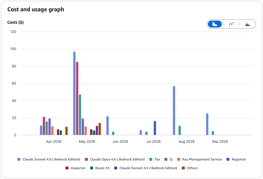
Now you look at the AWS bill. And you realize that Bedrock does not come for free. Bedrock caching also does not come for free and can be quite expensive, so sometimes semantic caching is a way to shrink your bill.
When to apply
Applicable wherever the same information is requested in different wordings and answering it is expensive, for example:
- LLM calls (RAG answers, chat, summaries)
- expensive database joins or aggregations
- paid external API calls
- compute-intensive search or scoring pipelines
Can semantic caching speed up RAG?
The RAG architecture is also using embeddings, so this is as fast as it gets. So, no speedup here. But the summarize or reranking part also costs tokens, and you can save that tokens with semantic caching.
Core idea
Classic caching uses an exact key (string equality or hash). That works for
deterministic lookups (user_id=42, sku=ABC123) but fails for natural-language
or freely phrased queries: the same intent is written many different ways, and
every variant misses the exact cache.
Semantic caching replaces exact key equality with proximity in vector space. Each query is turned into an embedding (vector). A new query is a hit when its cosine similarity to an earlier query exceeds a threshold. “Close enough in vector space” means “close enough in meaning” — then the cached answer can be reused and the expensive call avoided.
Query
  │
  ▼
generate embedding
  │
  ▼
search for most similar stored query
  │
  ├── similarity >= threshold ──► HIT: return cached answer
  │
  └── similarity <  threshold ──► MISS: run the expensive call,
                                   store (embedding, answer),
                                   return fresh answer
The entire benefit hinges on two knobs: the threshold and the vector store. Too low a threshold → “similar but wrong”. Too high → almost no hits. Both are calibrated empirically (the “Choosing thresholds” section).
Underlying assumptions
These assumptions MUST be checked per project — they decide whether, and how much, caching helps.
-
Recurring intents. There are enough queries with the same meaning but different wording. Without repetition there is no benefit. Directly measurable (share of queries with a near neighbor).
-
Deterministic / stable answers. The answer must not change during the cache period. If the underlying data changes (price update, policy change, inventory), a cached answer becomes wrong. Mitigation: TTL and targeted invalidation (the “Operations” section).
-
Similarity correlates with answer interchangeability. Two queries with similarity >= threshold should genuinely deserve the same answer. This is a modeling assumption, secured through calibration.
-
Thresholds are model- AND domain-specific. The cosine distribution of an embedding model is not universal. A 0.95 threshold for model A does not correspond to the same semantic distance for model B. Always calibrate against a ranked list of real pairs; never adopt a value blindly.
-
Embedding consistency (no drift). All vectors must come from the same model and the same configuration (dimension, normalization). Changing the model makes old and new vectors incomparable and forces a full re-embedding of the cache.
-
Normalized vectors. If embeddings are normalized to unit length, the dot product is already the cosine similarity — this makes comparison cheap and numerically stable.
-
Genuine repeat vs. double-logging. Two near-identical entries close together in time are often the same interaction (logged twice), not a real repeat hit. A hit counts only if it occurs at least N minutes after the first occurrence (recommended: 15 min). This prevents overestimating savings.
-
The first hit is always a miss. The first query of a cluster fills the cache (full call). Only later repetitions save. Savings therefore count repetitions, not unique queries.
-
Cold vs. warm cache. Looking at a time window in isolation (e.g. one month) understates savings with a “cold” cache, because clusters already known before the window are counted as misses. The “warm” cache (persisting across windows) is the realistic upper bound. Best to report both values.
-
Infrastructure cost is small compared to the expensive call. Embedding and vector-storage costs are typically orders of magnitude below the cost of the expensive call (e.g. an LLM). The business case rises and falls with the number of avoided calls, not with the cache infrastructure.
-
Privacy / tenant isolation. If answers are tenant- or user-specific, the cache key must include the tenant — otherwise another party’s answer is served. Semantic proximity alone is then not sufficient.
Analysis path (step by step)
How to determine, for any project, how much semantic caching would save — before building it in production.
-
Collect data. Export historical queries, at minimum
id, query_text, timestamp. The timestamp is mandatory for the repetition and time-window logic (assumptions 7–9). -
Deduplicate and aggregate metadata. Build a stable key per normalized text (lowercased, collapsed whitespace), e.g. SHA-256 of the normalized text. Per unique text, count all occurrences and record first/last seen — this later separates genuine repeats from double-logging.
-
Generate embeddings. Embed each unique query with one model. Concurrently (worker pool) and idempotently/resumably: skip queries already embedded — saves time and cost on a re-run.
-
Persist vectors. Store them. If a database already exists, it is often enough to add a vector attribute to the existing table — no new infrastructure required.
- Offline analysis: a full scan + in-memory comparison is enough.
- Production lookup with many vectors: use a real vector search (e.g. pgvector, OpenSearch k-NN, a dedicated vector DB), because a full scan per request becomes too expensive.
-
Compute pairwise similarity. Load all vectors and compute the cosine similarity of every pair. The naive comparison is O(n²); parallelize and use a float32 dot product. Keep only pairs above the lowest threshold to save memory (for n in the tens of thousands this is millions to billions of comparisons, but only a few relevant pairs).
-
Calibrate thresholds. Inspect the top-pairs list ranked by similarity and decide at which similarity pairs genuinely deserve the same answer. Set that threshold (often around 0.90–0.95); it is model-/domain-specific (assumption 4). The Levenshtein distance per pair helps distinguish trivial typo duplicates (distance 1–2) from real content variants.
-
Form clusters. Group queries transitively connected via >= threshold using union-find. One cluster shares exactly one cached answer.
-
Count cache hits (with the time rule). Sort occurrences per cluster by time: first occurrence = miss (fills the cache), every later occurrence
=
gap-minafterwards = hit. Optionally filter to a window (e.g. one month) and express percentages relative to the original number of queries in that window (not relative to unique queries). -
Compare costs.
- Savings = hits × cost per expensive call. The most defensible basis is a known total bill for the window divided by the number of queries (avoids token/volume estimates).
- Added cost = one-time embedding + additional vector storage (+ operating cost of the lookup, if any).
- Net = savings − added cost. Also report an upper bound with a warm cache (assumption 9) so the range is clear.
Choosing thresholds correctly
- There is no universally correct value. Calibrate against real pairs. In the real life example it was near 95% similariry.
- Rule of thumb from practice: higher threshold for sensitive topics (billing, contract, legal), where a “similar but wrong” answer is costly; slightly lower threshold for non-critical FAQ.
- Metrics when sweeping across thresholds: hit rate (rises as the threshold drops) vs. wrong-answer rate (also rises). Pick the point where the hit rate is still high but the wrong-answer rate is acceptably low.
- The Levenshtein distance as an extra signal: very small distance at high vector similarity ⇒ a pure typo/transposition ⇒ a safe cache hit.
Two text-comparison algorithms: Levenshtein distance vs. cosine similarity
The analysis uses two complementary algorithms to compare query texts. They measure fundamentally different things, and using both avoids each one’s blind spot.
Levenshtein distance (lexical / surface level). The minimum number of
single-character edits — insertions, deletions, substitutions — to turn one
string into the other. It operates on characters, knows nothing about
meaning, and is computed directly from the two texts (no embedding needed). It is
cheap: O(len_a × len_b) with two rolling rows.
- Distance 0 = identical text; distance 1–2 = a typo, a added/removed punctuation mark, a changed word ending.
- Example (same meaning, tiny edit): “Who is Spider-Man?” vs. “Who is Spiderman?” → distance 1 (the hyphen).
- Blind spot: it treats paraphrases as far apart. “Who is Iron Man?” and “What is Tony Stark’s superhero identity?” share almost no characters, so the distance is large even though the meaning is identical.
Cosine similarity (semantic level). The cosine of the angle between the two embedding vectors. It operates on meaning (as captured by the embedding model), not characters. For unit-normalized vectors it is simply the dot product. It needs an embedding per text but then is a cheap vector operation.
- 1.0 = same direction (same meaning); lower = less related.
- Example (different words, same meaning): the two Iron Man / Tony Stark questions above score high cosine similarity even though their Levenshtein distance is large.
- Blind spot: it can rate two different questions as fairly similar just because they share a topic (e.g. “Who is Thor?” vs. “Who is Loki?” — both about Asgardians), and the absolute scale is model-specific (assumption 4).
Why use both. Cosine similarity decides whether two queries mean the same thing — it is the primary gate for a cache hit. Levenshtein distance then qualifies the match: at high cosine similarity, a small Levenshtein distance confirms a trivial typo/wording variant (very safe to cache), whereas a large distance at the same similarity means a genuine paraphrase (still cacheable, but worth eyeballing during calibration). In short:
| Levenshtein distance | Cosine similarity | |
|---|---|---|
| Compares | characters (surface form) | meaning (embedding vectors) |
| Needs an embedding? | no | yes |
| Catches typos / punctuation | yes | yes |
| Catches paraphrases (different words) | no | yes |
| Cost | O(len_a × len_b) per pair | O(dim) per pair (dot product) |
| Role here | secondary signal / sanity check | primary hit decision |
Rule of thumb: gate on cosine similarity, sanity-check with Levenshtein. A pair with high cosine similarity and low Levenshtein distance is the safest possible cache hit; high cosine similarity with high Levenshtein distance is a real paraphrase and the most valuable case semantic caching exists for.
Cost model (template)
Savings           = cache hits  × cost_per_expensive_call
  cost_per_call   = known_total_bill / number_of_queries        (preferred)
                    OR (input_tokens × price_in + output_tokens × price_out)

Added cost        = embedding_one_time + vector_storage_per_month
                    (+ write cost, if vectors are newly persisted)

Net savings       = Savings − Added cost
Warm-cache bound: clusters already known before the window count every
                  in-window repetition as a hit.
Typical outcome: the added cost (embedding + vector storage) is negligible; the net savings correspond almost entirely to the avoided expensive calls. What matters is the realistic hit rate (cold vs. warm).
Operations: invalidation and drift (do not forget)
- TTL: every cache entry needs a lifetime matching the volatility of the data. If facts change, stale answers must not remain valid indefinitely.
- Targeted invalidation: on a known change (e.g. a topic area, a product), be able to delete the affected entries specifically — not just wait for TTL.
- Model / drift migration: when switching the embedding model, recompute all vectors; old and new are otherwise incomparable (assumption 5). Plan this migration before swapping the model.
- Short/ambiguous queries: very short inputs sit close to almost anything in vector space and produce false hits. Enforce a minimum length, or answer such queries directly, bypassing the cache.
- Monitoring: continuously observe hit rate, wrong-answer samples, and response latency; the threshold is not “set once and forget”.
Reference building blocks (optional template)
An example implementation of this methodology (Go + Amazon Bedrock Titan embeddings + DynamoDB) consists of small, interchangeable building blocks:
| Building block | Responsibility |
|---|---|
| CSV / data reader | reading, normalizing, stable IDs, timestamp aggregation |
| Embedding client | generate one vector per query (model easily swappable) |
| Vector store | add a vector attribute to the existing table, scan/lookup |
| Analysis | parallel similarity comparison, clustering, time-window hit logic, report |
| Union-find | transitive clusters above >= threshold |
| Levenshtein | character edit distance as an extra signal |
| Cost model | savings vs. infrastructure; prices as parameters |
Swap points for other projects:
- Embedding model: any model that returns normalized vectors (local or API). Re-embed after a switch.
- Vector store: DynamoDB with a native vector index (
SearchVectors,COSINE), an existing DB with a vector attribute, pgvector, OpenSearch k-NN, or a dedicated vector DB. - “Expensive call”: need not be an LLM — any costly, deterministic computation or query step.
AWS architecture — analysis solution (offline)
AWS architecture of the offline analysis solution: a Client reads results.csv into a Go program that performs the in-memory n x m cosine comparison, calls Amazon Bedrock Titan Embeddings v2 to embed queries, and uses Amazon DynamoDB (existing table plus a vector attribute) to store and bulk-load the vectors.
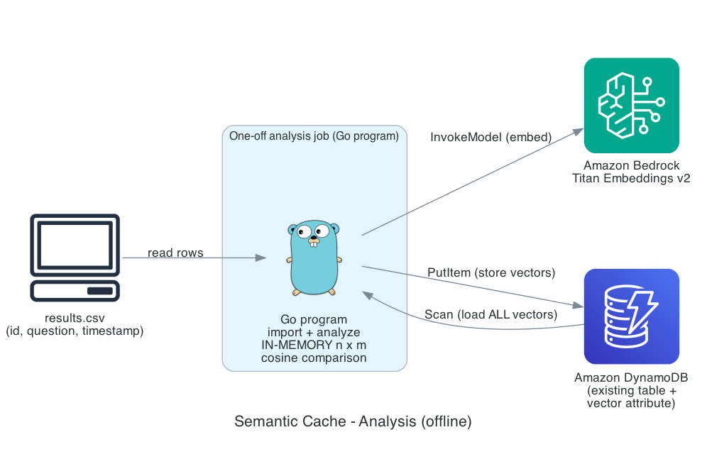
The analysis is a one-off, offline job. Its whole purpose is to measure how much
traffic is cacheable before anything is built into production. The key design
point: the similarity step compares every query vector against every other one,
i.e. n × m similarity comparisons. This is an O(n²) all-pairs problem and
should not run in the database. DynamoDB’s native vector index
(SearchVectors) does approximate nearest-neighbor for one query vector at
a time — great for the production lookup, but to materialize every pair for
the analysis you would issue n ANN queries, which is slower, costlier, and
approximate. Instead, for this exact all-pairs analysis, load all vectors once
and compare them in memory (parallelized, float32 dot product). The database
is used only as durable storage for the vectors.
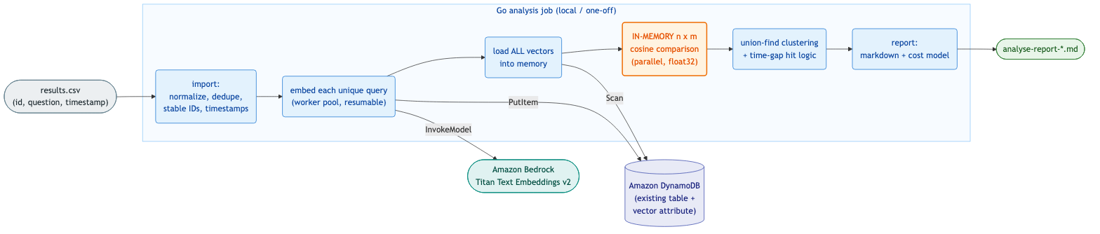
Why in memory, not in the database:
- All-pairs, not point lookups. The analysis needs every pairwise similarity (n × m). A vector index answers “nearest neighbors of one query” fast, but running that n times to materialize all pairs is far more expensive than a single in-memory sweep.
- Data size is small enough. A float32 vector of d dimensions is d × 4 bytes (1024 dims ≈ 4 KB). Tens of thousands of vectors fit comfortably in RAM (e.g. 50k × 4 KB ≈ 200 MB). The O(n²) sweep over ~12k vectors (~77M pairs) runs in under a minute on a laptop.
- Database stays a store. DynamoDB only persists the vectors (one
Scanto load them). No per-pair round trips.
Code snippet — read/write to DynamoDB (Go)
The vector lives as an embedding attribute (a DynamoDB list of numbers) on the
item, next to the question and timestamp metadata.
// Item is one question + its embedding, stored on the existing table.
type item struct {
    ID        string    `dynamodbav:"id"`
    Question  string    `dynamodbav:"question"`
    Embedding []float64 `dynamodbav:"embedding"` // DynamoDB "L" of "N"
    FirstSeen string    `dynamodbav:"first_seen,omitempty"`
    LastSeen  string    `dynamodbav:"last_seen,omitempty"`
    Count     int       `dynamodbav:"occurrences,omitempty"`
}

// WRITE one vector (upsert by id).
func (s *store) put(ctx context.Context, it item) error {
    av, err := attributevalue.MarshalMap(it)
    if err != nil {
        return fmt.Errorf("marshal item: %w", err)
    }
    _, err = s.client.PutItem(ctx, &dynamodb.PutItemInput{
        TableName: aws.String(s.table),
        Item:      av,
    })
    return err
}

// WRITE only metadata (cheap UpdateItem; does NOT touch the embedding).
func (s *store) updateMeta(ctx context.Context, id, firstSeen, lastSeen string, count int) error {
    _, err := s.client.UpdateItem(ctx, &dynamodb.UpdateItemInput{
        TableName:        aws.String(s.table),
        Key:              map[string]types.AttributeValue{"id": &types.AttributeValueMemberS{Value: id}},
        UpdateExpression: aws.String("SET first_seen = :f, last_seen = :l, occurrences = :c"),
        ExpressionAttributeValues: map[string]types.AttributeValue{
            ":f": &types.AttributeValueMemberS{Value: firstSeen},
            ":l": &types.AttributeValueMemberS{Value: lastSeen},
            ":c": &types.AttributeValueMemberN{Value: fmt.Sprintf("%d", count)},
        },
    })
    return err
}

// READ all vectors once (paginated Scan) -- the DB is used only as storage.
func (s *store) scanAll(ctx context.Context) ([]item, error) {
    var items []item
    var startKey map[string]types.AttributeValue
    for {
        out, err := s.client.Scan(ctx, &dynamodb.ScanInput{
            TableName:         aws.String(s.table),
            ExclusiveStartKey: startKey,
        })
        if err != nil {
            return nil, err
        }
        var page []item
        if err := attributevalue.UnmarshalListOfMaps(out.Items, &page); err != nil {
            return nil, err
        }
        items = append(items, page...)
        if out.LastEvaluatedKey == nil {
            break
        }
        startKey = out.LastEvaluatedKey // next page
    }
    return items, nil
}
Code snippet — in-memory vector comparison (Go)
After one scanAll, all vectors are compared in memory. They are
pre-normalized to float32 once, so cosine similarity is a plain dot product. The
outer loop is sharded across workers; each worker scans only the upper triangle
(j > i) to avoid computing every pair twice.
This step needs no third-party or AWS packages — only the Go standard
library: math for the vector norm (math.Sqrt),
and sync plus
runtime to run the comparison in parallel across
runtime.NumCPU() worker goroutines.
import (
    "math"    // math.Sqrt for the L2 norm
    "runtime" // runtime.NumCPU() to size the worker pool
    "sync"    // sync.WaitGroup to join the workers
)

// 1) normalize every vector once, into float32 (unit length => dot == cosine).
vecs := make([][]float32, n)
for i := range items {
    v := items[i].Embedding
    var norm float64
    for _, x := range v {
        norm += x * x
    }
    norm = math.Sqrt(norm)
    fv := make([]float32, len(v))
    for k, x := range v {
        fv[k] = float32(x / norm)
    }
    vecs[i] = fv
}

// 2) parallel all-pairs sweep; `rows` is a channel of row indices i.
go func(p *partial) {
    for i := range rows {
        vi := vecs[i]
        for j := i + 1; j < n; j++ { // upper triangle only
            sim := dot32(vi, vecs[j]) // cosine, because vectors are unit length
            if sim >= t95 {
                p.near95[i], p.near95[j] = true, true
                p.hi95 = append(p.hi95, pair{I: i, J: j, Similarity: float64(sim)})
            }
        }
    }
}(p)

// 3) the hot inner product: a tight float32 loop.
func dot32(a, b []float32) float32 {
    var s float32
    for i := range a {
        s += a[i] * b[i]
    }
    return s
}
AWS architecture — production solution (online)
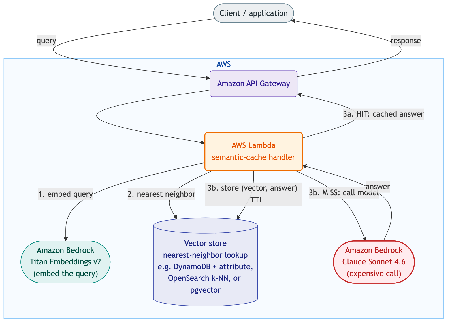
AWS architecture of the online production solution: a Client calls Amazon API Gateway, which invokes an AWS Lambda semantic-cache handler. The handler embeds the query with Amazon Bedrock Titan Embeddings v2, looks up the nearest neighbor in an Amazon DynamoDB vector cache (with TTL and per-tenant partitioning); on a cache hit it returns the cached answer, on a miss it calls Amazon Bedrock Claude Sonnet 4.6 and stores the new vector and answer.
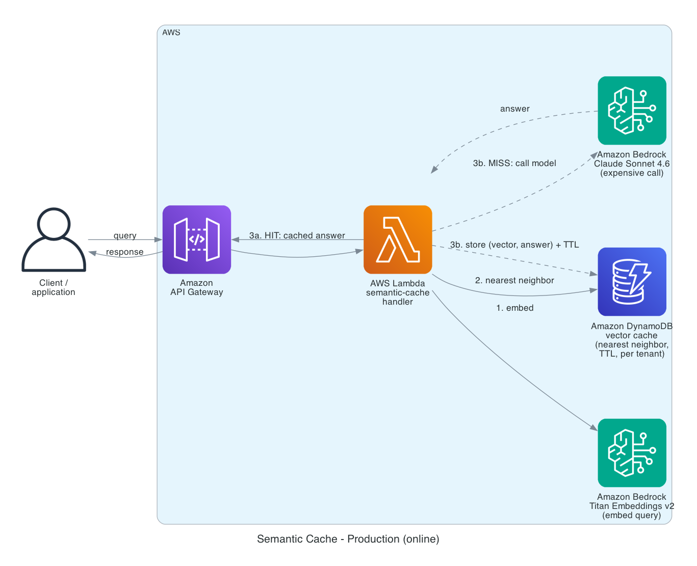
In production the cache sits in front of the expensive model call. Each incoming query is embedded, the single nearest cached entry is looked up, and on a hit the stored answer is returned without calling the LLM. Here the lookup is a point query (nearest-neighbor), not all-pairs, so a vector index is appropriate.
Production notes:
- Vector store choice depends on volume. DynamoDB has native vector
indexes (approximate nearest-neighbor search via the
SearchVectorsAPI with aCOSINEdistance function), so for most volumes the vectors and the nearest-neighbor lookup both live in DynamoDB — no separate vector store. For very large or specialized workloads, Amazon OpenSearch k-NN, pgvector on Amazon RDS/Aurora, or a dedicated vector DB are alternatives. - TTL + invalidation (the “Operations” section) live on the cache entries.
- Tenant isolation (assumption 11): partition the lookup by tenant.
- Threshold from the offline analysis (the “Choosing thresholds” section) is the gate for hit vs. miss.
Production flow
Cost comparison — Bedrock, 100 calls (Sonnet 4.6 vs. Titan v2)
All figures use Amazon Bedrock on-demand list prices only:
- Claude Sonnet 4.6: $3.00 per 1M input tokens, $15.00 per 1M output tokens.
- Claude Sonnet 5.5: $2.00 per 1M input, $10.00 per 1M output.
- Claude Opus 5.5: $4.00 per 1M input, $20.00 per 1M output.
- Amazon Titan Text Embeddings v2: $0.02 per 1M tokens ($0.00002 per 1k).
Realistic token profile for one RAG-style call:
- Input ≈ 2,000 tokens — a short user question (~20 tokens) plus the retrieved context/clauses and the system prompt that a RAG call sends to the model.
- Output ≈ 800 tokens — a long answer with citation blocks.
- Embedding input ≈ 20 tokens — only the question text is embedded, not the retrieved context.
Per call:
| Item | Tokens | Rate (Bedrock) | Cost per call |
|---|---|---|---|
| Sonnet 4.6 input | 2,000 | $3.00 / 1M | $0.006000 |
| Sonnet 4.6 output | 800 | $15.00 / 1M | $0.012000 |
| Sonnet 4.6 total | $0.018000 | ||
| Titan v2 embedding | 20 | $0.02 / 1M | $0.00000040 |
For 100 calls:
| Scenario | Cost (100 calls) |
|---|---|
| 100 × Claude Sonnet 4.6 (no cache) | $1.80 |
| 100 × Titan v2 embedding only | $0.00004 |
| Ratio (Sonnet / Titan per call) | ~45,000 × |
Model comparison — same token profile (2,000 input / 800 output), different Claude model on the expensive call:
| Model | Input / 1M | Output / 1M | Cost / call | 100 calls |
|---|---|---|---|---|
| Claude Sonnet 5.5 | $2.00 | $10.00 | $0.012000 | $1.20 |
| Claude Sonnet 4.6 | $3.00 | $15.00 | $0.018000 | $1.80 |
| Claude Opus 5.5 | $4.00 | $20.00 | $0.024000 | $2.40 |
| Titan v2 (embedding) | $0.02 | — | $0.00000040 | $0.00004 |
The more capable (and expensive) the model on the uncached call, the more each cache hit saves: a hit on Opus 5.5 saves ~$0.024, on Sonnet 4.6 ~$0.018, on Sonnet 5.5 ~$0.012 — while the Titan embedding that enables the hit costs the same ~$0.0000004 regardless. Caching is therefore most valuable in front of the priciest model.
Reading of the result:
- One Sonnet 4.6 RAG call (~$0.018) costs about 45,000 times one Titan embedding (~$0.0000004). The embedding needed to decide a cache hit is effectively free next to the model call it can avoid.
- Therefore every cache hit saves ~$0.018 and the semantic-cache machinery (embedding + vector lookup) costs a tiny fraction of a single avoided call. Even a modest hit rate pays for the whole mechanism many times over.
- Note the output tokens dominate the Sonnet bill (here $0.012 of $0.018, i.e. two thirds). Long answers make caching more valuable, because each avoided call saves the expensive output generation.
Prices are Amazon Bedrock on-demand list prices and can change; verify current rates on the AWS Bedrock pricing page and your own Cost Explorer. Batch mode (−50%) and prompt caching (up to −90% on repeated input) are separate Bedrock levers that reduce the Sonnet baseline further but do not change the semantic cache’s value proposition.
Scaled cost and speed savings (real-world example)
The token counts below come from a real-world example — a production question/answer log (insurance-domain RAG), reported as aggregated token statistics.
Measured token profile (real-world example):
| Quantity | Measured | Used here |
|---|---|---|
| Question tokens (user input) | mean ~15, median ~13, p90 ~25 | 20 |
| Answer tokens (model output, incl. citations) | mean ~638, range 350–1050 | 650 |
| Sonnet input per call (question + retrieved context + system prompt) | — | 2,000 |
Per-call cost (Amazon Bedrock on-demand list prices):
| Item | Tokens | Rate | Cost / call |
|---|---|---|---|
| Claude Sonnet 4.6 input | 2,000 | $3.00 / 1M | $0.006000 |
| Claude Sonnet 4.6 output | 650 | $15.00 / 1M | $0.009750 |
| Sonnet 4.6 per call | $0.015750 | ||
| Titan v2 embedding | 20 | $0.02 / 1M | $0.00000040 |
Cost normalized to 1k / 10k / 100k queries
Baseline = every query hits Sonnet (no cache). Embedding cost is the one-time cost to embed all queries (negligible).
| Queries | Sonnet 4.6 baseline (no cache) | Titan embeddings (all) |
|---|---|---|
| 1,000 | $15.75 | $0.0004 |
| 10,000 | $157.50 | $0.0040 |
| 100,000 | $1,575.00 | $0.0400 |
| 1,000,000 | $15,750.00 | $0.4000 |
Cost savings by cache hit rate
Savings = (hit rate × queries) avoided Sonnet calls − embedding cost. The embedding cost is so small it barely moves the result, so savings scale almost exactly with the hit rate. Three illustrative hit rates are shown: 5%, 10%, and 37% (the figure reported in the source article).
| Queries | Baseline | Save @ 5% | Save @ 10% | Save @ 37% |
|---|---|---|---|---|
| 1,000 | $15.75 | $0.79 | $1.57 | $5.83 |
| 10,000 | $157.50 | $7.87 | $15.75 | $58.27 |
| 100,000 | $1,575.00 | $78.71 | $157.46 | $582.71 |
| 1,000,000 | $15,750.00 | $787.10 | $1,574.60 | $5,827.10 |
Real-world example — measured cacheable percentage. On the actual data (August 2026, the >= 95% similarity cluster with the >= 15-minute repeat rule) the measured cacheable share was 5.2% with a cold cache and 9.7% with a warm cache (clusters already seen before the month). Applying those real rates:
| Queries | Baseline | Save @ 5.2% (cold) | Save @ 9.7% (warm) |
|---|---|---|---|
| 1,000 | $15.75 | $0.82 | $1.53 |
| 10,000 | $157.50 | $8.19 | $15.28 |
| 100,000 | $1,575.00 | $81.90 | $152.78 |
| 1,000,000 | $15,750.00 | $819.00 | $1,527.75 |
Net savings ≈ gross savings, because the embedding + storage cost (see the “Cost comparison” section) is a tiny fraction of even a single avoided call.
Speed savings (latency)
Caching also removes latency: a hit returns the stored answer after only the embedding call plus the vector lookup — on the order of ~0.2 s — instead of a full generation. For this example an uncached question takes up to 20 s.
Time saved per cache hit = uncached latency − cache response (~0.2 s):
| Uncached answer latency | Cache hit latency | Time saved per hit | % faster | Speedup |
|---|---|---|---|---|
| 1 s | ~0.2 s | ~0.8 s | ~80% | ~5× |
| 10 s | ~0.2 s | ~9.8 s | ~98% | ~50× |
| 20 s | ~0.2 s | ~19.8 s | ~99% | ~100× |
| 30 s | ~0.2 s | ~29.8 s | ~99% | ~150× |
“% faster” = time saved ÷ uncached latency; “Speedup” = uncached latency ÷ cache hit latency. A cache hit is near-instant, so beyond a few seconds of uncached latency the response is essentially ~99% faster.
Aggregate time saved = (time saved per hit) × (number of cache hits). Example at the measured 20 s latency: 10,000 queries × 10% hit rate = 1,000 hits × ~19.8 s ≈ ~5.5 hours of generation time avoided, and those users get a near-instant answer. The longer the uncached answer takes, the larger both the cost saving (more output tokens) and the latency saving per hit.
Whats next
If you need consulting to support your AWS development, your Amazon Connect Customer or GenAI project, don’t hesitate to contact us, tecRacer.
Want to learn Go on AWS? Go here
Thanks to
This blog post has been supported by AI.
Foto von Vladimir Fedotov auf Unsplash