Hyperparameter Tuning with Ray 2.x and AWS Sagemaker
In this blog post, we will talk about hyperparameter tuning using Ray’s RLlib and Sagemaker. This should serve as an add-on to a previous blog post on Ray 2.x and Sagemaker.
Background
When setting up a machine learning model training (for example a neural network), we can configure many parameters beforehand. These parameters, which cannot be directly learned from the data during the model training, are called hyperparameters. If you are already familiar with deep learning, you would know that the hyperparameter space can be extremely large. As an example, we can vary the learning rate, the number of layers, batch size, regularization parameters and a lot more. Each of these parameters has a large configuration space, and the space of the cartesian product is even larger. To make things more complex, each algorithm can have its own additional set of hyperparameters as well.
Why do we care about these hyperparameters? Our task is to optimize a training objective, this could be minimizing a loss function or maximizing the reward in reinforcement learning tasks, and the choice of hyperparameters is an essential part of this optimization task. As mentioned earlier, we cannot grasp this large space and most of the time will not understand a priori which parameters will lead to a better final result. That’s why we need to start several trainings with many sets of varying hyperparameters to find an optimal one. This process is called hyperparameter tuning.
Let’s focus on the actual task, namely reinforcement learning on AWS Sagemaker using Ray’s RLlib. Assuming the reader is familiar with the blog post mentioned previously, we want to perform a so-called hyperparameter sweep on a reinforcement learning task. More precisely, we want to start a lot of training jobs with different hyperparameters to find a good set of them.
Here we encounter some practical problems: First, reinforcement learning trainings can take a long time to converge. Performing hyperparameter tuning with a lot of trainings, especially in the cloud (we often need to use GPU-based instances), can incur a lot of costs. Secondly, for reinforcement learning, we have a lot more hyperparameters to configure compared to a simple neural network or a classical machine learning algorithm. Therefore, trying to find the optimal parameters is not efficient at all. In short, our task is to perform hyperparameter tuning while keeping costs low.
Hyperparameter Tuning on Sagemaker
Luckily, Sagemaker provides us with a Tuner class, which we can use to perform exactly that. Additionally, Sagemaker also makes it extremely straightforward to perform training with spot instances while managing interruptions for us. What makes the combination of Ray and Sagemaker here wonderful is the fact that when an interrupted training is restarted, Ray will simply pick up the latest checkpoint and resume training.
Let’s dive into the specifics, we will extend the code from the previously mentioned blog post to perform trainings using hyperparameter tuning.
First, we will define the hyperparameter tuning configuration:
OBJECTIVE_METRIC = "episode_reward_mean"
MAX_JOBS = 2
MAX_PARALLEL_JOBS = 1

hyperparameter_ranges = {
                         "rl.training.config.lr":{"min_value":0.000001,"max_value":0.01},
                         }

hyperparameter_tuning = {
                         "hyperparameter_ranges": hyperparameter_ranges,
                                                   "objective_metric":OBJECTIVE_METRIC,
                                                   "max_jobs":MAX_JOBS,
                                                   "max_parallel_jobs":MAX_PARALLEL_JOBS
                        }
The specific structure of the hyperparameters is derived from the experiment configuration structure of Ray experiments.
Before we can instantiate the Tuner class, we need to make a few additional imports:
from sagemaker.tuner import HyperparameterTuner
from sagemaker.parameter import (
    ContinuousParameter,
    CategoricalParameter,
    IntegerParameter,
)
The second import is important, we need to define what space the tuner should search for and what type each parameter is. For example, the learning rate is a continous parameter, so we need to wrap the previously defined hyperparameter range using the ContinousParameter class:
hyperparameter_ranges[key] = ContinuousParameter(
                    min_value=val["min_value"], max_value=val["max_value"]
                )
Of course, this should be done for every tunable hyperparameter, so we need to add some logic to read the previously defined hyperparameter dictionary and wrap them into the corresponding parameter classes:
hyperparameter_ranges = {}
for key, val in hyperparameter_tuning.get("hyperparameter_ranges", {}).items():
    if type(val) is dict:
        if type(val["min_value"]) is int:

            hyperparameter_ranges[key] = IntegerParameter(
                min_value=val["min_value"], max_value=val["max_value"]
            )
        else:
            hyperparameter_ranges[key] = ContinuousParameter(
                min_value=val["min_value"], max_value=val["max_value"]
            )
    if type(val) is list:
        hyperparameter_ranges[key] = CategoricalParameter(val)
Finally, we can define the Tuner class (assuming we already have an estimator defined, see the previous blog post) and perform a fit, which starts the training in Sagemaker:
tuner = HyperparameterTuner(
                    estimator=estimator,
                    objective_metric_name=hyperparameter_tuning.get("objective_metric", "episode_reward_mean"),
                    hyperparameter_ranges=hyperparameter_ranges,
                    metric_definitions=metric_definitions,
                    max_jobs=hyperparameter_tuning.get("max_jobs", 1),
                    max_parallel_jobs=hyperparameter_tuning.get("max_parallel_jobs", 1),
                )
tuner.fit(wait=False)
That’s it! The tuner will try to find a good set of hyperparameters using a Bayesian strategy (more on the different types of strategies here). Think of the Bayesian strategy as one in which we use prior training results to make a more educated guess on where to look next. That’s why for this particular strategy it makes sense to run the jobs sequentially (for example five sequential blocks à two parallel trainings). Before we show some screenshots of the Sagemaker Hyperparameter Tuning dashboard, we should enable spot training to reduce costs (remember we will start a lot of trainings to find good hyperparameters). As promised, this is a simple argument passed to the estimator class:
use_spot_instances=True,
What will we see in Sagemaker? As soon as we start the tuning job, the following appears in the hyperparameter tuning dashboard:

We have started two sequential blocks with two parallel trainings, so after these two trainings are done the next block will be started. Let’s look at one specific training:
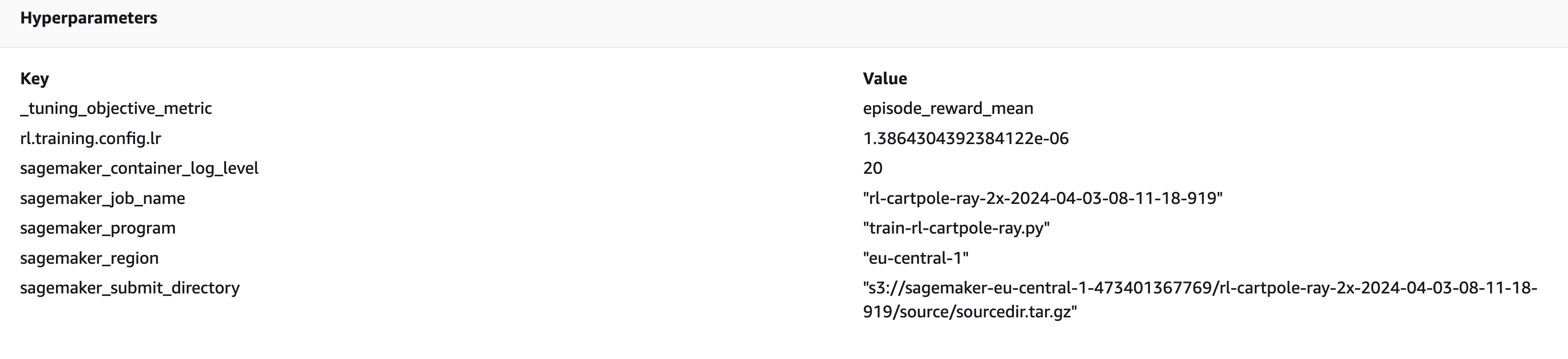
Note that we have only defined the learning rate as the hyperparameter, and we can see that Sagemaker has chosen a learning rate within the pre-defined range.
After all the trainings have finished, we can take a look at the best training job (that which has the highest mean episode reward out of all trainings):
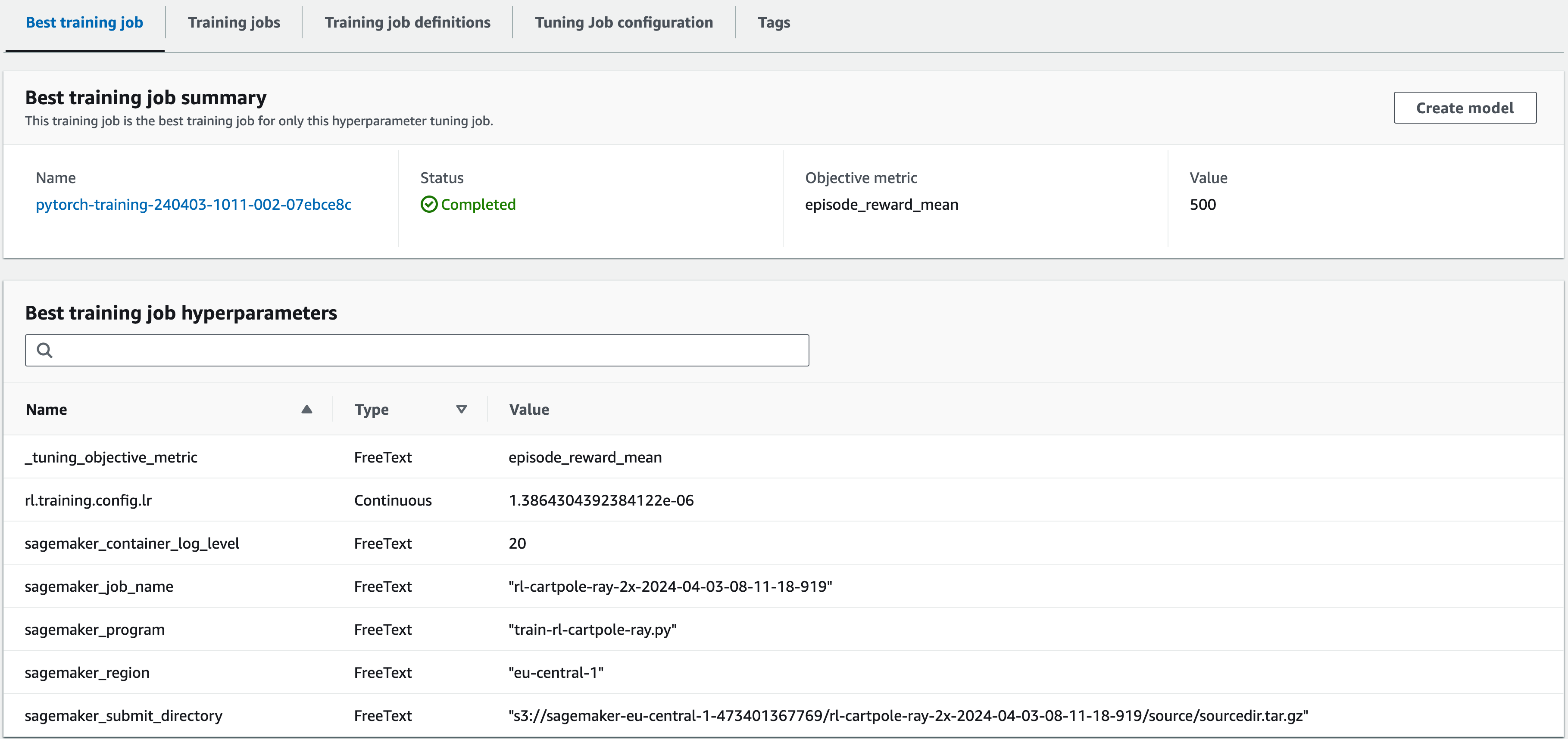
As you can see, Sagemaker automatically detects the best training job, this is especially useful if hyperparameter tuning is part of a Sagemaker Pipeline, in which subsequent steps can take the best training job and perform post-training tasks.
Finally, let’s look at the cost savings when using spot trainings for the best training job:
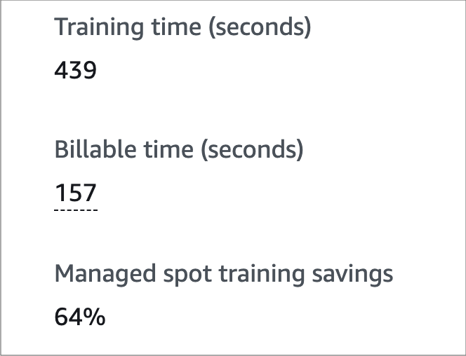
The total training time for this job was 439 seconds, but we were only billed for 157 seconds because we used a spot instance. We have managed to save 64% on training costs, a huge saving which will especially be noticeable when we train for much longer and with many more training jobs.
Summary
In this blog post, we have explored how to perform hyperparameter tuning for reinforcement learning models with Ray’s RLlib on Sagemaker using spot instances. We have seen the simplicity of starting multiple training jobs to find a good set of hyperparameters and managed to keep costs low by using managed spot trainings.
— Chrishon
See also
- Ray 2.x and Sagemaker
- Reinforcement learning in production using Ray and Amazon SageMaker
- Ray’s Rllib
Title Photo by Denisse Leon on Unsplash