Push-Down-Predicates in Parquet and how to use them to reduce IOPS while reading from S3
Working with datasets in pandas will almost inevitably bring you to the point where your dataset doesn’t fit into memory. Especially parquet is notorious for that since it’s so well compressed and tends to explode in size when read into a dataframe. Today we’ll explore ways to limit and filter the data you read using push-down-predicates. Additionally, we’ll see how you can do that efficiently with data stored in S3 and why using pure pyarrow can be several orders of magnitude more I/O-efficient than the plain pandas version.
Your first impulse to solve the memory allocation problem may be reading and filtering the data. Still, client-side filtering can be challenging in a memory-constrained environment like a Lambda function. Client-side filtering often requires the data to fit into memory. That means you can’t limit the data size because it’s too large to fit into memory - a classic Catch-22. Let’s look at some techniques that can actually help you solve this problem.
To understand how these work, it’s helpful to understand more about the internal structure of Parquet files and how these support so-called “push-down-predicates” (we’ll get back to those later). I will try to give a summary here. There is an excellent blog by Peter Hoffmann that goes into more detail if you’re curious.
In a nutshell, Parquet is a hybrid of a row-oriented and columnar data storage format. The file is divided into Row Groups, which are - you guessed it - groups of rows. Within each group, the data is stored in a column orientation, i.e., the values for each column are stored sequentially. This enables better compression and more efficient reading of data for OLAP workloads. Parquet also keeps statistics about each row group, such as the min/max value for each column, in the footer of the file. Here’s a simplified example of what that looks like.
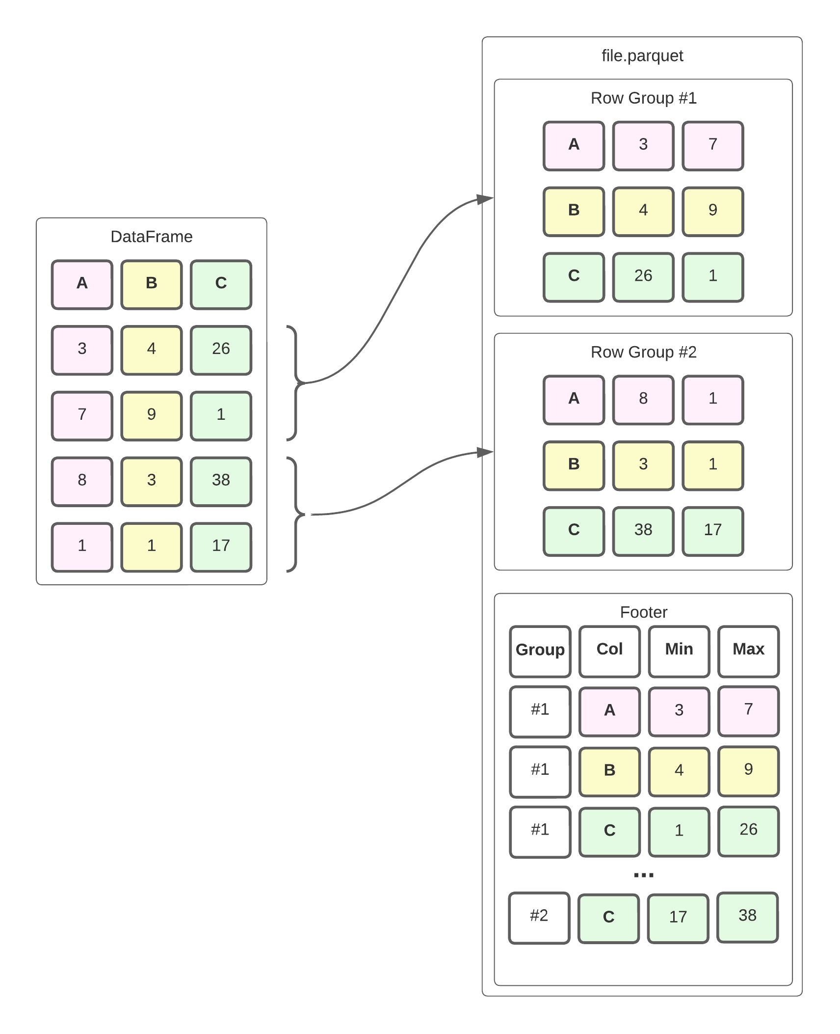
The dataframe is divided into row groups, which store the values of each column within it sequentially. The footer stores metadata such as the minimum and maximum for each column in the row group. In reality, the file format is slightly more complex, but this is a good enough mental model to help us understand how we can efficiently read this data.
Suppose we want to compute the equivalent of this SQL query, i.e., the sum of all values in column b for rows where c > 30:
select sum(b)
  from data_frame
 where c > 30
If this were a CSV file, we’d read the whole file into a dataframe, filter on column c, and then aggregate on column b. We’d also have to read column a, although we don’t need it to compute the desired result. This is because CSVs are row-oriented and less sophisticated data structures. Often I/O operations are comparatively expensive, so reading more data than necessary is not ideal when dealing with non-trivial amounts of data.
Fortunately, Parquet is a more sophisticated file format that allows us to perform fewer I/O operations to answer the query. When we read the file, we immediately look at the metadata in the footer to determine which row groups and columns we need. Conveniently we can ignore all row groups where max(C) < 30, which means we’d only read row group 2 in our example. Additionally, the metadata allows us to jump directly to the values for columns B and C in row group 2. This means we won’t even read the values for column A. This is what push-down predicates are. They allow us to push some filter criteria down to the reader, potentially reducing the I/O and the system memory required to store the data.
How can we do this in Python? Fortunately, that’s pretty easy, and we even have two different ways of doing that. The first is the built-in support for push-down predicates in pandas, and the second option is using pyarrow to read the parquet file and convert it to a pandas dataframe. Usually, pandas will use pyarrow to read parquet files anyway (although it can also use fastparquet).
Let’s look at some examples and data to see how that helps. If we want to use pyarrow to implement our query from above, the implementation will look something like this:
import pandas as pd
import pyarrow.dataset as ds

path_to_parquet = "s3://bucket/object.parquet"

dataframe: pd.DataFrame = ds.dataset(path_to_parquet, format="parquet").to_table(
	columns=["b"],
	filter=ds.field("c") > 30
).to_pandas()
The pandas version looks very similar. The key difference here is that the parameter is called filters instead of filter.
import pandas as pd
import pyarrow.dataset as ds

path_to_parquet = "s3://bucket/object.parquet"

dataframe: pd.DataFrame = pd.read_parquet(
	path_to_parquet,
	columns=["b"],
	filters=ds.field("c") > 30
)
Note that we also rely on the pyarrow filter expression since pandas passes down the filter to the underlying pyarrow implementation. To learn more about the possible filter options, check out the pyarrow expression documentation. Both implementations also allow you to chain filters for more complex expressions, e.g.:
dataframe: pd.DataFrame = ds.dataset(path_to_parquet, format="parquet").to_table(
	columns=["b"],
	filter=ds.field("c") > 30 & ds.field("c") < 40 & ds.field("b").isin([1, 2])
).to_pandas()
So what’s the difference between the two implementations, and why would you choose one over the other? Both implementations can read data from S3, but how they do this differs. The pandas implementation relies on the additional dependency s3fs that provides a file-system-like API to S3. If you use pyarrow directly, you benefit from the built-in S3-support in the underlying Arrow C++ implementation. This frees you from having to ship additional dependencies with your code.
By playing around with the two different implementations, I also learned a few more performance details that surprised me. Let’s talk a bit about my experiment setup. The complete code is also available on GitHub if you want to follow along.
First, I generated a sample dataframe with 2 million rows that looks something like this:
| category | number | timestamp | uuid |
|---|---|---|---|
| blue | 3.33 | 2022-10-01T05:00:00+00:00 | abd32d… |
| red | 7 | 2022-10-01T05:00:00+00:00 | def32d… |
| gray | 20000.65 | 2022-10-01T05:00:00+00:00 | aed31d… |
| blue | 3.33 | 2022-10-01T05:00:00+00:00 | cb452d… |
The four columns contain the following data:
categorywith the string valuesblue,red, andgraywith a ratio of ~3:1:2numberwith one of 6 decimal valuestimestampthat has a timestamp with time zone informationuuida UUID v4 that is unique per row
I sorted the dataframe by category, timestamp, and number in ascending order. Later we’ll see what kind of difference that makes. The first three columns should compress quite well since they have few distinct values. In fact, the parquet file without the uuid column would be about 1.9 MByte in size. The uuid column is mainly added to simulate less relevant data and create a decently sized parquet file. After the dataframe is generated, the parquet file is uploaded to S3 - it is about 64.5 MBytes in size. Additionally, I set the row group size to 200k rows so that each chunk of data is about 5% of the total data.
We must develop a few filter conditions test scenarios now that we have our test data. I decided to read only the columns category, number, and timestamp from the Parquet and used the following filter criteria.
full frameshould return all rows, i.e., there is no filtercategory == 'blue', which should yield about half of the rowscategory in ('red', 'gray'), which should return the other half of the rowsnumber <= 8.24, which should result in about 40% of the datatimestamp <= '2022-10-03T17:00:00+12:00', which should return about half of the datatimestamp <= '2022-10-03T17:00:00+12:00' & category == 'blue', which should yield roughly a third of the data.
I implemented each filter in the pandas and pyarrow styles and ensured that each implementation’s results were identical. For each test case, I used psutil to measure the network bandwidth the operation consumed. I measured both bytes sent and received, but the former didn’t amount to significant numbers, so let’s focus on the amount of data read.
The following chart compares the performance of both implementations regarding the amount of data received. Less is better here. The x-Axis is scaled logarithmically, which means each vertical line increases the scale by a factor of 10. This is the only way these numbers could be sort of visually compared. I also compared the kibibytes received when working with a sorted (see above) vs. an unsorted dataset.
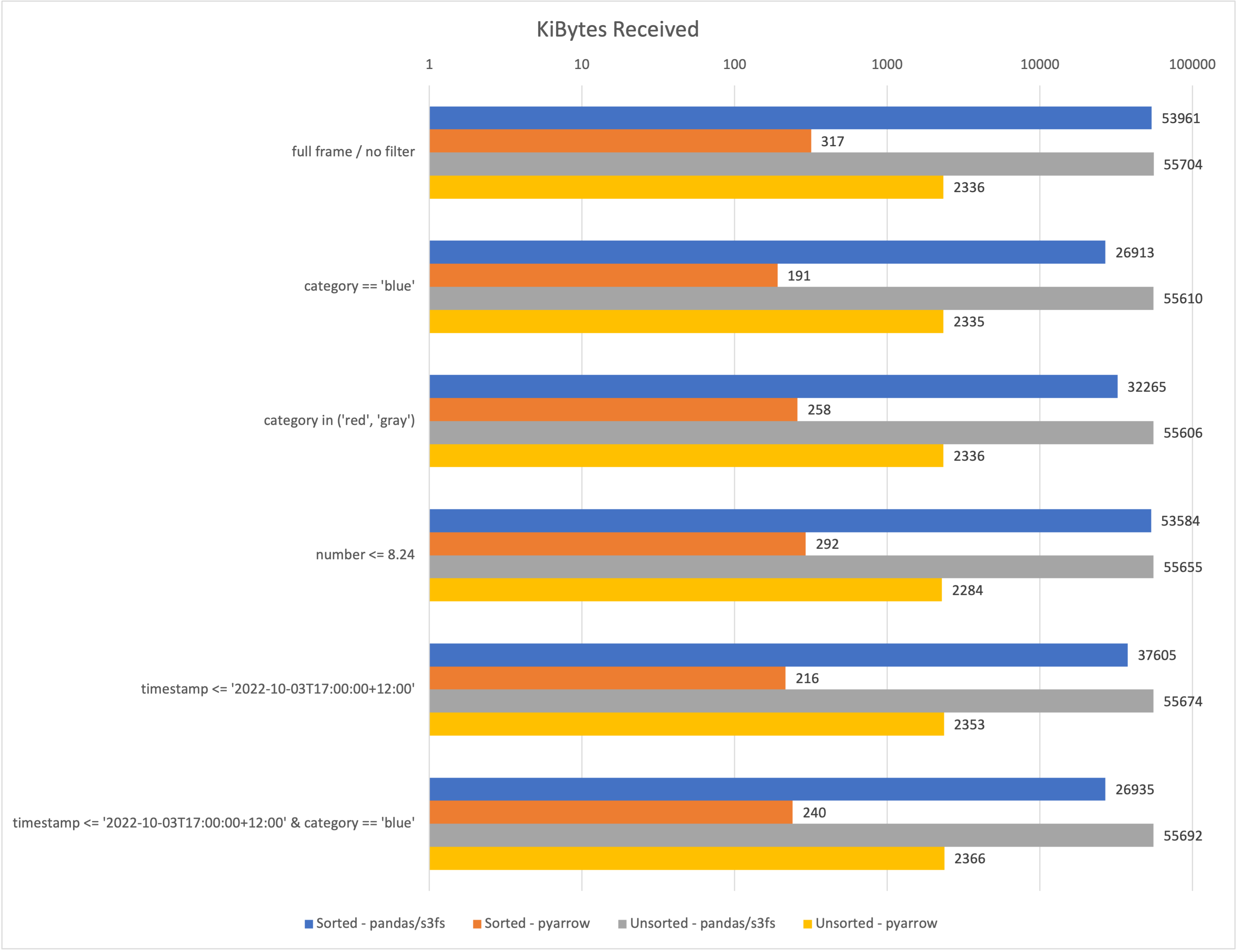
In all cases, I only requested three of the four columns, reducing the downloaded data by at least a few Megabytes. Although the effectiveness of the filtering differs significantly between the pandas and pyarrow implementations. Here are some of my key takeaways:
- On average, the
pyarrowimplementation reads several orders of magnitude less data than thepandas/s3fsimplementation. - When using the
pyarrowversion, sorting the data can significantly reduce the amount of data read. - It seems that the Arrow/C++ implementation is a lot more efficient than the
s3fsversion.
Of course, these findings come with a few caveats.
- I/O is only one of the multiple dimensions in the trade-off you must consider regarding performance.
- When reading tiny amounts of data, i.e., < 2MB parquet files, I sometimes observed the
pandas/s3fsto download slightly less data. Realistically this won’t affect you when you’re at the point where you want to read-optimize your code. - When using either of the options to read parquets directly from S3, I couldn’t mock S3 buckets using
moto. There may be some way to force that with the s3fs version, but I couldn’t get it running. - (I have a lingering suspicion which I can’t get rid of, that I did something wrong with the s3fs version. Feel free to check the code and let me know if I need to correct it.)
Conclusion
We learned a bit about the internal structure of parquet files and how that can be leveraged to reduce the I/O required when we only need to work with a subset of the data. We explored the two primary ways this can be implemented when working with pandas and learned that it’s usually a good idea to go with the pyarrow implementation since that is faster and uses fewer dependencies.
Hopefully, you learned something new. I’m looking forward to your feedback on any of the social media channels listed in my bio. If you like this content, chances are you’d also like doing data analytics projects with our help.
— Maurice